
If your workload follows a pattern, waiting for CPU alarms is often too late. I’d use forecast-led scaling to add capacity before the rush, then keep reactive autoscaling in place for anything the model misses.
Here’s the short version:
- Reactive scaling lags. In Kubernetes, new capacity can take 2–4 minutes to become ready.
- Predictive scaling fits repeat demand. It works best for things like 09:00 weekday sign-ins, month-end reporting, and payroll runs.
- History matters. AWS can start with 24 hours of data, but 14 days is a better baseline for weekly patterns.
- Signal choice matters too. Queue depth, request backlog, and active sessions often tell you more than CPU alone.
- Most teams should use a hybrid setup. A simple rule is: Final replicas = max(reactive, predictive).
- Put limits around spend. Use hard budget caps, replica bounds, hold-down windows, and a manual override path.
If I were putting this into practice, I’d keep the plan simple:
- Measure full scale latency, including warm-up time.
- Pick signals that show demand early.
- Forecast the baseline for known peaks.
- Let HPA, KEDA, or cloud autoscaling catch surprise spikes.
- Review forecast error and idle spend after each incident or code change.
::: @figure 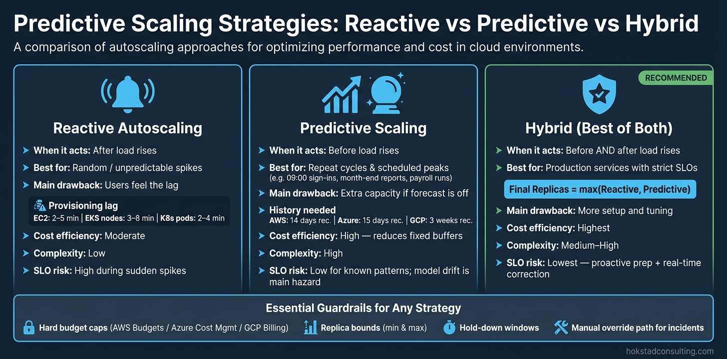 {Reactive vs Predictive vs Hybrid Scaling: Cost, Performance & Complexity}
:::
{Reactive vs Predictive vs Hybrid Scaling: Cost, Performance & Complexity}
:::
Lightning Talk: Predictive Autoscaling in Kubernetes With KEDA and Prophet - Snigdha Kanchana, IBM
Need help optimizing your cloud costs?
Get expert advice on how to reduce your cloud expenses without sacrificing performance.
Quick comparison
| Approach | When it acts | Best for | Main drawback |
|---|---|---|---|
| Reactive autoscaling | After load rises | Random spikes | Users may feel the lag |
| Predictive scaling | Before load rises | Repeat cycles and scheduled peaks | Extra capacity if the forecast is off |
| Hybrid | Before and after load rises | Production services with strict SLOs | More setup and tuning |
The core idea is simple: don’t scale from panic if you can scale from pattern.
Foundations: Metrics, forecasting methods and workload patterns
Workload signals that drive better forecasts
The metrics you feed into a forecasting model matter just as much as the model itself. CPU utilisation helps, but it usually tells you what has already happened. It’s a lagging signal.
Leading indicators give you earlier warning. Queue depth, such as SQS queue length or Kafka topic lag, HTTP request backlog, and active session counts show demand that’s building up before it fully hits your workers. CPU, memory, request rate, and p95 latency still matter too. When you choose better signals, you cut wasted headroom and reduce the risk of service degradation.
Two practical rules make a big difference:
- Collect metrics at 30-second to 1-minute intervals. Coarser data can hide short spikes in your training set [1].
- Tag deployment events in your metrics pipeline. New code often changes resource behaviour, so old baselines can stop being useful. After a deployment, expect 1–3 days before the model settles into a stable baseline again [1].
These signals only help if they line up with the workload pattern your forecast is meant to model.
Forecasting methods: from simple trends to machine learning
The next step is turning those signals into a forecast you can use. There isn’t one method that fits every workload. The best option depends on how much historical data you have, how messy the demand pattern is, and how much engineering time you want to spend.
| Method | Typical fit | Data Requirements | Implementation Complexity | Cost planning fit |
|---|---|---|---|---|
| Simple Trends | Low | Minimal (hours) | Low | Good for stable, linear growth |
| Holt-Winters or ARIMA | Medium | Moderate (days) | Medium | Suitable for clear daily/weekly seasonality |
| ML (Prophet, LSTM) | High | High (2–4 weeks) | High | Best for complex, multi-variable demand patterns |
For most teams, Holt-Winters or ARIMA is a sensible starting point because both handle daily and weekly seasonality well. ML-based methods such as Prophet or LSTM networks can be more accurate for complex, multi-variable demand patterns, but they need more historical data and regular retraining. A common rhythm is daily retraining for high-traffic services and weekly retraining for steadier ones, so accuracy doesn’t quietly drift over time [1][4].
In early 2026, Palo Alto Networks cut Kubernetes scaling incidents by 45% after moving from static threshold automation to an autonomous ML-based predictive system that learned from outcomes instead of human-tuned thresholds [1].
Once you have a forecast, the next job is mapping it to the scaling layer that can act on it.
Autoscaling building blocks across cloud and Kubernetes
A forecast only matters if the scaling mechanism can use it. So the scaling primitive you choose matters just as much as the forecast itself. Each option scales something different, reacts at a different speed, and suits a different kind of workload.
Horizontal scaling means adding more instances or pod replicas. That’s the default choice for stateless, bursty workloads such as web APIs. In Kubernetes, the Horizontal Pod Autoscaler (HPA) does this job, although standard HPA can still take 2–4 minutes to react to a spike [1].
Vertical scaling changes the CPU and memory allocated to existing pods or VMs instead of adding more of them. The Kubernetes Vertical Pod Autoscaler (VPA) works well for stateful applications or workloads with unpredictable memory use. One catch: don’t run VPA and HPA on the same workload unless VPA stays in recommendation-only mode. If not, pod restarts can throw replica counts off balance [1].
For event-driven or queue-based workloads, KEDA is often the better fit. It scales pods from external signals such as Kafka topic lag or SQS queue depth, so it can act before CPU or memory pressure shows up. For VMs, Google Cloud Managed Instance Groups need 3 days of history and use CPU only for prediction. Load balancing and custom Cloud Monitoring metrics aren’t supported [5].
| Scaling Mechanism | Best For |
|---|---|
| Horizontal (HPA) | Bursty, stateless web traffic - scales by adding replicas |
| Vertical (VPA) | Stateful apps or unpredictable memory needs - scales by resizing pods |
| KEDA | Queue-driven or event-driven workloads (e.g., Kafka lag, SQS depth) |
| Scheduled / Cron | Highly predictable batch jobs or known daily peaks |
Designing predictive scaling strategies across AWS, Azure, GCP and Kubernetes
Using native predictive scaling features effectively
Once you’ve picked the right signals and built the model, the next step is simple in theory and tricky in practice: connect that forecast to the platform that will act on it. The goal isn’t to keep extra capacity sitting around all day. It’s to bring in just enough capacity early enough to handle the load.
Native predictive scaling works a bit differently across the main cloud providers. AWS and Azure forecast scale-out only, while GCP can forecast both scale-out and scale-in.
AWS EC2 Auto Scaling creates a 48-hour forecast and refreshes it every 6 hours. It can work with as little as 24 hours of history, though 14 days is recommended for better accuracy [8]. It supports CPU, network, and custom CloudWatch metrics [8]. The SchedulingBufferTime setting controls how far ahead instances launch, which is a big deal if your app needs several minutes to initialise [8][10].
Azure predictive autoscale for VM Scale Sets uses a 24-hour forecast window. It needs at least 7 days of history, with 15 days giving the best results [10]. It works from average CPU only. You can also choose a 5–60 minute pre-launch window [10].
GCP predictive autoscaling for Managed Instance Groups needs 3 days of history, with 3 weeks recommended for better accuracy [5]. It recomputes its forecast every few minutes and is the only one here that supports both scale-out and scale-in [5]. The catch? It only works with CPU utilisation, so custom metrics aren’t supported [5]. There’s also no separate charge for GCP predictive autoscaling; you only pay for the VMs [5].
Start in forecast-only mode first. That gives you time to compare the prediction with live traffic before you let the platform add or remove capacity on its own [8][10][5].
| Platform | Min. History | Forecast Window | Pre-launch Range | Metrics Supported | Scale-in? |
|---|---|---|---|---|---|
| AWS EC2 | 24 hours (14 days rec.) [8] | 48 hours [8] | Customisable via SchedulingBufferTime [8]
|
CPU, Network, Custom CloudWatch metrics [8] | No [8] |
| Azure VMSS | 7 days (15 days rec.) [10] | 24 hours [10] | 5–60 minutes [10] | CPU (average) only [10] | No [10] |
| Google Cloud MIGs | 3 days (3 weeks rec.) [5] | Recomputed every few minutes [5] | Based on initialisation period [5] | CPU only [5] | Yes [5] |
Predictive approaches for Kubernetes workloads
Kubernetes needs a different setup because it scales pods, not instances. Standard HPA reacts after demand goes up, which leaves a 2–4 minute lag before new pods are ready [1].
A good pattern is to pair a forecast-driven baseline with HPA or KEDA as the reactive safety net. In practice, that means using a forecasting model - Prophet or an LSTM network trained on 2–4 weeks of history - to adjust the minReplicaCount in a ScaledObject or HPA spec ahead of known demand cycles [4][1]. The forecast lifts minReplicaCount, and HPA or KEDA deals with the spike you didn’t see coming.
The signal you choose matters a lot. For web APIs, requests per second is a better leading indicator than CPU [9]. For background workers and async pipelines, queue depth or consumer lag should lead the way - for example, Kafka topic lag or SQS queue depth [1][9].
You also need to protect shared downstream systems. If the app tier shares a database, cap maxReplicas. App pods can scale much faster than the database can handle new connections. Using a connection multiplexer such as PgBouncer or RDS Proxy, along with a hard replica ceiling, helps protect the data tier [9].
Turning strategy into code and operating practice
Treat forecast retraining like any other production job. Trigger it after material deployments or after sustained forecast drift [1]. When a major deployment lands, tag the change and retrain the model, because old baselines stop matching new behaviour [1].
Then review forecast error, buffer timing, and signal lag after each incident or idle-capacity run.
Cost forecasting, trade-offs and governance
Scenario planning for cloud cost projections
Turn forecast demand into spend before you set scaling rules. Start by mapping expected load to instance, pod or GPU counts. Then multiply that by the unit cost. For budgeting, use the 90th-percentile cost band from your forecast distribution instead of a cheerful average. That gives finance teams a more realistic upper limit [7].
This gets much more useful when you add scenarios. Percentile-based planning helps you judge each demand event by risk, then match it to the right response.
| Scenario | Resource Pattern | Cost Overrun Risk | Recommended Tactic |
|---|---|---|---|
| 10% month-on-month growth | Linear, predictable increase | Low | Standard ML-based predictive scaling with monthly model retraining [3] |
| Product launch | Sharp, non-linear step-up | High | Event multipliers + manual pre-scaling + reactive backup [3][6] |
| AI inference rollout | High GPU demand, token-based | Very High | Capacity planning on tokens/sec; model tiering and strict instance caps [3] |
| Seasonal peak (e.g. Black Friday) | Extreme cyclical spike | Critical | Historical pattern analysis; 90th percentile confidence bands; manual overrides [3][11] |
Before you lock in any policy, replay past demand through the scaling rules and compare the projected spend. It’s a low-risk way to stress-test the model against real traffic before it goes anywhere near production [7][11].
Reactive versus predictive scaling: cost and performance trade-offs
Reactive autoscaling is easy to run, but it comes with a hidden bill: provisioning lag. EC2 instances usually need 2–5 minutes to come online, and EKS node groups take 3–8 minutes [3]. In that gap, requests either sit in a queue or fail.
Predictive scaling moves the cost elsewhere. You spend more engineering time on model upkeep and tuning. But it can be well worth it when cold starts hurt - like large ML models or JVM-based services - or when holding idle buffer capacity costs too much [7][11].
For most teams, a hybrid setup is the safest default: predictive scaling for the baseline, reactive scaling for the odd spike or miss.
| Approach | Cost Efficiency | Performance During Spikes | Complexity | Best Fit |
|---|---|---|---|---|
| Reactive | Moderate - idle waste when buffers are held | High SLO risk during sudden spikes [3][11] | Low | Stable, slow-moving workloads |
| Predictive | High - reduces fixed buffers | Low risk for known patterns; model drift is the main hazard [11][7] | High | Seasonal or bursty traffic |
| Hybrid | Highest | Lowest - proactive prep plus real-time correction [11][7] | Medium–High | Production systems with strict SLOs |
Once you can see the cost and performance trade-off clearly, the next job is putting firm limits around it.
Governance, budgets and risk control
Keep forecasting separate from actuation so you can change, pause or roll back either one on its own [11]. Set hard spend caps in your cloud provider’s budgeting tools - AWS Budgets, Azure Cost Management, or GCP Billing Budgets. Then wire alerts at 80% and 95% of the threshold so both finance and engineering get warning before things drift too far.
Just as important, operators need a fast manual override. They should be able to pin replica count or disable predictive actions instantly during an incident [11].
The governance model shapes ownership and risk appetite:
| Feature | Central FinOps Governance | Team-Owned Scaling Policies |
|---|---|---|
| Primary goal | Global budget compliance | Service performance and SLOs |
| Control mechanism | Platform-wide spend caps | Custom metrics and local guardrails |
| Risk handling | Conservative; prioritises savings | Aggressive; prioritises availability |
| Audit path | Centralised cost dashboards | Per-service observability logs |
Most organisations end up somewhere between the two. Central teams set spend guardrails, and service teams own the scaling logic inside those limits.
With forecasts, trade-offs and guardrails in place, rollout starts to look less like guesswork and more like day-to-day operations.
Conclusion: A practical roadmap for predictive scaling
Treat predictive scaling like an operating loop: measure, forecast, act, review. It works as a continuous cycle, not a one-time switch.
The hard part usually isn’t the model. It’s how fast your system can respond once a forecast says, “scale now”.
Start with your scale latency - the full time from a scaling decision to a pod being ready to serve traffic. That includes node provisioning, image pulls, and application warm-up, such as cache hydration [11][12]. This number matters because it tells you how much spare capacity you need sitting there in advance. And that, in plain terms, affects what you pay to avoid delays.
Once you know how long a service takes to warm up, choosing a forecasting method gets much simpler. It becomes a matching exercise, not guesswork. Use schedules for fixed peaks, statistical models for regular seasonality, and ML only when demand is highly variable or deployments shift the baseline [1][4].
When forecasts are live in production, accuracy matters just as much as raw capacity. Track prediction error, and use MAE to catch systematic over-forecasting before it turns into avoidable spend. After major deployments, retrain or adjust the model, because new code can change resource consumption patterns fast enough to make an earlier forecast go stale [1][2].
The safest starting point is usually a hybrid policy. Let predictive scaling set the baseline capacity curve, and let reactive autoscaling handle surprise spikes. A good default rule is Final Replicas = max(Reactive, Predictive) [12][7].
It also helps to put guardrails around the whole setup:
- Conservative scale-down
- Hold-down windows
- Minimum and maximum replica bounds
- A manual override path for incidents [11][7]
For support linking forecasting to scaling automation, Hokstad Consulting can help with cloud cost engineering and DevOps automation.
FAQs
When should I use predictive scaling?
Use predictive scaling when your workload follows stable, repeating demand patterns that show up clearly in past data. That could mean daily office-hour traffic, weekly usage swings, or seasonal peaks.
It works especially well for apps with long start-up or warm-up times. In those cases, reactive scaling can kick in too late and lead to latency or performance problems. Hokstad Consulting recommends predictive scaling as a way to cut over-provisioning and get capacity in place before traffic arrives.
Which metrics are best for forecasting demand?
The best metrics are the ones that line up with your workload and the things that move your business. Start with the core infrastructure numbers: CPU utilisation, memory use, network throughput, and response time. They give you a solid baseline.
Then layer in application metrics such as active user sessions, queue depth, Kafka topic lag, or HTTP request backlogs. If it fits your setup, bring in business indicators too. For example, you might look at cost per 1,000 requests alongside performance signals like p95 latency.
That mix gives you a clearer picture of what’s happening, both at the system level and in terms of spend and user experience.
How do I start with hybrid scaling safely?
Start with a phased approach built around observability and risk reduction. The first step is to run predictive scaling in forecast-only mode. That way, it can make recommendations without changing capacity, which gives you room to compare predicted capacity against actual demand before anything goes live.
When the forecasts are holding up well, let predictive scaling handle baseline capacity and keep reactive autoscaling in place as a safety net for sudden spikes. Track accuracy with MAPE, along with the gap between predicted and actual usage, and review your policies and limits on a regular basis.