
When building models to predict cloud spending, not all data points are useful. Including irrelevant features can harm accuracy and increase costs. Feature selection helps you focus on the most important variables, like instance types or workload patterns, improving model performance while reducing complexity.
Here are five methods to refine your dataset for better forecasts:
- Variance Threshold: Removes features with little variation, ideal for eliminating constant or near-constant values.
- Correlation-Based Filtering: Identifies and removes highly correlated features to reduce redundancy.
- Mutual Information: Detects nonlinear relationships between features and the target variable.
- Recursive Feature Elimination (RFE): Uses a model to iteratively rank and remove less important features.
- Embedded Feature Selection: Integrates feature selection directly into model training, such as Lasso regression or tree-based methods.
Each method has its strengths and limitations, making them suitable for different stages of cloud spend forecasting. For large datasets, start with quick filters like Variance Threshold or Correlation Filtering. For high-dimensional data with complex interactions, techniques like RFE or Embedded Selection offer deeper insights.
Quick Comparison
| Method | Best For | Cost | Limitation |
|---|---|---|---|
| Variance Threshold | Removing static/noisy features | Very Low | Ignores target variable relationships |
| Correlation-Based Filtering | Tackling redundant metrics | Low | Misses nonlinear patterns |
| Mutual Information | Nonlinear feature relevance | Moderate | Struggles with sparse/high-dimensional data |
| Recursive Feature Elimination (RFE) | Precise feature subset selection | High | Computationally expensive for large datasets |
| Embedded Selection | High-dimensional data with feature interactions | Moderate | Model-dependent results |
Choosing the right method depends on your dataset size, model needs, and business goals. Start simple, and scale to advanced techniques for larger cloud budgets or complex datasets.
::: @figure 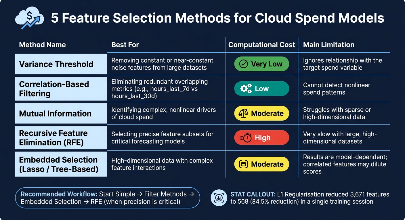 {5 Feature Selection Methods for Cloud Spend Models: Quick Comparison}
:::
{5 Feature Selection Methods for Cloud Spend Models: Quick Comparison}
:::
1. Variance Threshold
Variance thresholding is one of the simplest methods for feature selection. The concept is easy to grasp: calculate the variance of each feature and remove those that fall below a chosen threshold. Features with little to no variance are essentially constant across the dataset, meaning they add almost no value to predictive modelling.
In cloud billing data, repetitive columns are more common than you might think. For example, fields like Billing Currency, Billing Account ID, or Availability Zone in a single-region setup may have the same value in every row. These static features provide no useful signal for identifying cost drivers.
Best Use Case
Variance thresholding is particularly effective as an initial filtering step for large billing datasets, especially when many columns are constant or nearly constant. By eliminating these redundant features early, you simplify the dataset and make further analysis faster. However, it's a good idea to scale numerical features before applying this method. Metrics like hourly cloud usage can vary widely in scale, and without scaling, features measured in larger units might seem to have high variance purely due to their size, not because they’re meaningful.
Computational Cost
One of the biggest perks of variance thresholding is its speed. Since it calculates variance for each feature independently and doesn’t factor in the target variable (like monthly spend), there’s no need to train a model. This makes it an incredibly fast approach, even with datasets containing hundreds of features. That said, it’s worth noting that this method has its limits, which we’ll address next.
Main Limitation
The main drawback of variance thresholding is that it doesn’t consider how a feature relates to the target output. Because it’s unsupervised, it might discard low-variance features that are actually crucial for prediction. For instance, a rarely used but expensive service type could be eliminated, even though it has a significant impact on costs. To avoid this pitfall, variance thresholding should be paired with a supervised technique, like Mutual Information or Recursive Feature Elimination, to ensure no important features are missed.
2. Correlation-Based Filtering
After using variance thresholding to eliminate low-variance features, correlation-based filtering takes the process a step further by tackling redundancy. Unlike variance thresholding, which evaluates features individually, correlation-based filtering examines the relationships between features. The goal? To identify and remove features that are highly correlated, as they often provide overlapping information. Keeping both doesn't add value and can even hinder your model's performance.
The process is simple: calculate correlation coefficients for pairs of features and drop one if their absolute correlation exceeds a threshold, typically 0.8 or higher. For example, in cloud billing data, metrics like hours_last_7d and hours_last_30d often show correlations above 0.9. Retaining both introduces redundancy without improving insights. In regression models, this redundancy, known as collinearity, can destabilise coefficient estimates, leading to unreliable predictions [6].
Best Use Case
Correlation-based filtering is particularly effective as an initial step during exploratory data analysis (EDA). It’s ideal for datasets with numerous overlapping metrics, like cloud usage logs. When two features are flagged as redundant, it's wise to keep the one that's simpler or easier to interpret. For instance, prioritise raw usage counts over derived metrics to make your model more transparent for finance or engineering teams [3].
The choice of correlation metric is also critical. Use Pearson correlation for linear relationships between continuous numerical features. For non-linear relationships or ordinal data, consider Spearman or Kendall's tau [2][4]. This approach not only simplifies your dataset but also boosts computational efficiency.
Computational Cost
One of the advantages of correlation-based filtering is its speed. It scales well, even with large datasets containing millions of rows, because it’s a filter method. This means it operates independently of machine learning models, eliminating the need for training and keeping computational costs low [1].
Main Limitation
The biggest drawback of this method is its limited scope. Correlation-based filtering evaluates features in pairs, ignoring potential interactions within larger groups of features. A feature might seem redundant when compared to one other feature but could still be valuable in combination with others. As highlighted in Applied Predictive Modeling:
Most of these techniques are univariate, meaning that they evaluate each predictor in isolation. In this case, the existence of correlated predictors makes it possible to select important, but redundant, predictors.[5]
Additionally, Pearson correlation has its own constraints. It only captures linear relationships, so features with strong non-linear ties to the target variable might be overlooked. To address this, consider pairing it with methods like Mutual Information to uncover non-linear dependencies [7].
3. Mutual Information
When linear methods fall short, Mutual Information (MI) steps in as a powerful alternative. Unlike correlation-based filtering, which only captures linear relationships, MI can handle both linear and nonlinear dependencies. It measures how much knowing a feature reduces uncertainty about the target variable (in this case, cloud spend) [10]. This makes MI particularly useful for tackling the intricate and unpredictable patterns often seen in cloud billing data [9][11].
MI assigns a score to each feature, with zero indicating no relationship and higher scores reflecting stronger relevance to the target [8][10]. This ranking system allows you to identify the most important features before diving into model training.
Best Use Case
MI shines when the connection between cloud usage metrics and spend is unclear or nonlinear [8][9]. It works seamlessly with mixed data types, handling both discrete features (like service regions or instance types) and continuous variables (such as CPU utilisation or storage throughput) [13]. A key tip: ensure that each feature is properly classified as either discrete or continuous before running MI calculations. Misclassifying a feature can lead to inaccurate results [13].
Additionally, MI can act as a preprocessing filter, helping you eliminate irrelevant features before applying more resource-intensive methods. This can significantly speed up the rest of your modelling pipeline [14]. Incorporating MI into your feature selection process can improve efficiency and accuracy in forecasting cloud spend.
Computational Cost
MI estimation relies on non-parametric techniques, like k-nearest neighbour (k-NN) distance calculations, to estimate entropy without assuming a specific data distribution [8][13]. The computational complexity typically ranges from O(N log N) to O(N^(1+α)) as the dataset size increases [12]. For larger datasets, using tools that support parallel processing - such as the n_jobs parameter in scikit-learn - can help distribute the workload across multiple CPU cores, keeping processing times reasonable [8][13].
Main Limitation
MI does have its drawbacks. It struggles with data sparsity in high-dimensional datasets, where estimating accurate joint probability distributions becomes challenging. Histogram-based methods, in particular, may fail in such scenarios [15]. Another limitation is that MI, when applied pairwise, cannot detect synergistic interactions - cases where two features are only predictive when combined but appear irrelevant individually [16].
The accuracy of MI estimation also depends on hyperparameter choices, like the number of neighbours in k-NN methods. While increasing this value reduces variance, it can also introduce bias [8][9]. For extremely high-dimensional datasets, a practical workaround is to use two-dimensional approximations that balance relevance against redundancy [15]. This approach helps navigate MI's limitations while still leveraging its strengths.
4. Recursive Feature Elimination (RFE)
Recursive Feature Elimination (RFE) is a wrapper method that uses a machine learning model to determine which features should be retained. Unlike methods that evaluate features individually, RFE takes an iterative approach. It starts by training a model on the entire feature set, ranks the features based on their importance, removes the least significant ones, and then retrains the model on the reduced set. This process continues until the desired number of features remains.
The ranking of features depends on the metrics provided by the model. For instance, linear models use coef_ values, while tree-based models rely on feature_importances_. To ensure consistency, it's important to use the same model for RFE as the one planned for production since feature importance varies between models.
Best Use Case
RFE works well with datasets that have a high number of features and complex interactions - such as cloud spend data, where factors like usage hours, instance types, regional pricing, and time-based aggregates interact. For example, one case study reduced the number of features from 127 to 15, which led to an improvement in AUC from 0.836 to 0.851 and reduced training time from 47 minutes to just 90 seconds [6]. To avoid trial-and-error when deciding how many features to keep, RFECV (RFE with Cross-Validation) can be used. This variant automatically determines the optimal subset size based on cross-validation scores.
Computational Cost
The computational cost of RFE increases with the number of iterations, as the model needs to be retrained each time. To speed things up, you can increase the step size (removing multiple features per iteration) and leverage parallel processing. Applying a quick filter method, like Variance Threshold or correlation filtering, before running RFE can also help by removing irrelevant features early on.
Main Limitation
A key challenge with RFE is its tendency to focus on local optima. It might discard features that only become useful when combined with others [17]. For example, when two features carry overlapping information, their importance scores may be diluted, leading to the removal of one that could have been valuable [6].
RFE is recognised as a greedy search strategy, as it does not explore all possible feature combinations exhaustively but rather selects locally optimal features at each iteration.- Okan Bulut et al., University of Alberta [17]
With its iterative refinement approach, RFE provides a robust way to streamline feature selection. However, the next method takes this a step further by embedding feature selection directly into the model training process.
5. Embedded Feature Selection
Embedded feature selection weaves the selection process directly into model training, removing the need for extra steps before or after. Essentially, the algorithm determines which features to keep as it learns. This approach stands apart from pre-selection filters like Variance Threshold or post-training methods like RFE, offering a more streamlined process.
Two popular techniques include L1 regularisation (Lasso), which penalises less useful features by reducing their coefficients to zero, and tree-based methods, which rank features based on impurity reduction at decision tree nodes. For example, in one logistic regression pipeline, L1 regularisation automatically discarded 3,103 out of 3,671 features - an impressive 84.5% reduction - in just one training session [18]. By integrating feature selection with training, embedded methods provide an efficient alternative to the filter and wrapper approaches discussed earlier.
The main advantages are speed and simplicity: Since feature selection is implicitly performed during model fitting, no additional feature selection process needs to be added to the workflow, which tends to save a lot of computational time.- Master Machine Learning with scikit-learn [18]
Best Use Case
Embedded methods shine when dealing with large-scale datasets, such as those tracking cloud spending. These datasets often include high-dimensional and noisy feature spaces, like usage metrics, engagement ratios, and temporal aggregates. In these cases, embedded methods are often preferable to filter or wrapper techniques. If your features are highly correlated, consider using ElasticNet instead of Lasso to maintain predictive recall. Research across 134,400 simulated configurations revealed that in environments with high multicollinearity, Lasso's recall can drop to 0.18, while ElasticNet holds steady at 0.93 [20]. Also, remember to standardise your features before applying Lasso, as its L1 penalty is sensitive to the scale of the variables [7].
Computational Cost
The computational cost of embedded methods is minimal beyond the model training itself. This makes them the most efficient choice when you need interaction-aware selection without running countless iterations [18]. For tree-based models, consider replacing Gini importance with SHAP (SHapley Additive exPlanations) values. SHAP values provide more reliable feature attribution, especially for high-cardinality features such as instance types or region codes [7].
Main Limitation
The key limitation is model dependency: features selected for one model may not work well if you switch to another [6][18]. For example, if you move from linear regression to gradient boosting, you may need to reassess your feature set entirely. To enhance stability, run embedded selection across repeated cross-validation folds. Features that appear in 95% of folds are far more reliable than those showing up in just 20% [19].
Comparison Table
Here's a side-by-side look at the five methods, breaking them down by their best applications, computational demands, and primary drawbacks.
| Method | Best Use Case | Computational Cost | Main Limitation |
|---|---|---|---|
| Variance Threshold | Quick screening to eliminate constant or near-constant noise features | Very Low | Doesn't account for the relationship with the target spend variable [6] |
| Correlation-Based Filtering | Removing redundant cloud metrics (e.g., overlapping CPU usage metrics) | Low | Cannot detect nonlinear spend patterns [6] |
| Mutual Information | Identifying complex, nonlinear drivers of cloud spend | Moderate | Needs larger datasets for reliable results [21] |
| Recursive Feature Elimination (RFE) | Selecting the best feature subset for critical forecasting models | High | Very slow with large, high-dimensional datasets [6][22] |
| Embedded Selection | Works well for high-dimensional data where interactions between features are key | Moderate | Correlated features may dilute importance scores [23] |
This table highlights how each method fits into different stages of cloud spend forecasting. Start with fast, general-purpose filters to clear out noise, such as variance thresholding or correlation-based filtering. Methods like RFE are better suited for smaller datasets where precision matters, as they can be computationally intensive [22].
A key point to note: usage features like hours
and sessions
often display high multicollinearity. Applying correlation-based filtering early on can help address this issue effectively [6].
The curse of dimensionality is not a theoretical curiosity. It is a measurable, reproducible degradation in model performance that happens every time you include features that do not carry signal.- DataField.Dev [6]
For a balanced approach, start by trimming irrelevant features with fast filters, incorporate embedded selection during model training, and save RFE for when precision is the top priority.
Conclusion
Choosing the right feature selection method for your forecasting needs boils down to three key factors: the size of your dataset, your model's specific requirements, and the practical needs of your business.
If you're just starting out, it's smart to begin with straightforward approaches. Filter methods like Variance Threshold and Correlation-Based Filtering are excellent for large datasets. For organisations with a cloud spend under £40,000 per month, these methods are often enough. However, when your annual spend exceeds £400,000, more advanced techniques like embedded methods and Recursive Feature Elimination (RFE) become worthwhile. In such cases, even a modest 2–3% boost in forecast accuracy can justify the added engineering effort [24].
Here’s a quick guide:
- Use filter methods to eliminate noise in the data.
- Opt for embedded selection if you need a balance between speed and accuracy.
- Choose RFE when precision is critical, especially if you're working with smaller datasets.
For mature FinOps teams, hitting a Mean Absolute Percentage Error (MAPE) of under 15% for medium-term forecasts is a common goal. Structured feature selection plays a major role in achieving this benchmark [24].
A simpler model with better features will almost always outperform a complex model trained on noisy, irrelevant data.- HCL GUVI [25]
As cloud environments are constantly changing, retraining models quarterly and updating forecasts monthly is essential. This ensures your forecasts stay relevant as architectures evolve. Keep in mind that the importance of features can shift over time, and outdated selections might quietly harm the accuracy of your predictions without obvious signs [24].
FAQs
Which feature selection method should I start with for my cloud billing dataset?
Start with filter methods such as correlation or mutual information to quickly screen out features that are irrelevant or redundant. These methods are efficient and provide a solid starting point for narrowing down your dataset.
Next, explore SelectFromModel, which uses estimators capable of offering feature importance scores. This approach helps refine your selection by focusing on features that have a measurable impact on your model.
For a more detailed analysis, turn to SHAP-based methods. These techniques pinpoint the smallest set of features that significantly influence your model's performance, offering deeper insights into feature contributions.
How do I choose the right correlation threshold without losing important cost drivers?
To choose the right correlation threshold, aim to strike a balance between eliminating redundant data and keeping essential features. Prioritise features that show a strong correlation with your target spend metric, have higher variance, or contain fewer missing values. For linear models, it’s crucial to remove highly correlated features to avoid multicollinearity, which can make coefficients unstable. Hokstad Consulting supports businesses in fine-tuning their cloud environments, ensuring predictive models remain reliable and practical for managing costs effectively.
How often should I redo feature selection as my cloud environment changes?
Feature selection isn’t a one-and-done deal - it should be revisited whenever your model starts to show signs of drift or when notable changes occur in your cloud environment. In cloud-native setups, automated pipelines often address this during retraining cycles or when data drift is detected. However, if your production environment becomes unstable or features start shifting quickly, it’s a good idea to review your logic. Hokstad Consulting highlights the importance of this practice to ensure forecasts stay in sync with changing workloads and business metrics.