
Managing cloud costs can be challenging, but predictive analytics transforms this process into a data-driven, proactive strategy. By leveraging machine learning (ML) models, businesses can forecast expenses with up to 91.7% accuracy, identify trends, and reduce unexpected cost spikes. This method combines historical billing data with real-time metrics to refine predictions and improve financial planning.
Key insights include:
- Trend-based models: Use historical data to predict stable workloads, but may struggle with dynamic environments.
- Driver-based models: Focus on future business events like product launches or growth, offering better accuracy for fluctuating workloads.
- Hybrid strategies: Combine both models to balance past trends and future changes, keeping forecast variances as low as 10–12%.
For UK organisations, fluctuating currency rates and variable operating costs make accurate forecasting essential. Tools like AWS Cost Explorer, Amazon QuickSight, and DoiT Cloud Analytics can aid teams at different maturity levels. Regular reviews, collaboration across teams, and integrating cost optimisation efforts into forecasts are critical for success.
With predictive analytics, businesses can avoid budget overruns, align costs with goals, and improve decision-making across finance, engineering, and leadership teams.
Mastering Cost Predictability: Forecasting and Budgeting Strategies for Databricks
Need help optimizing your cloud costs?
Get expert advice on how to reduce your cloud expenses without sacrificing performance.
Trend-Based Forecasting Models
::: @figure 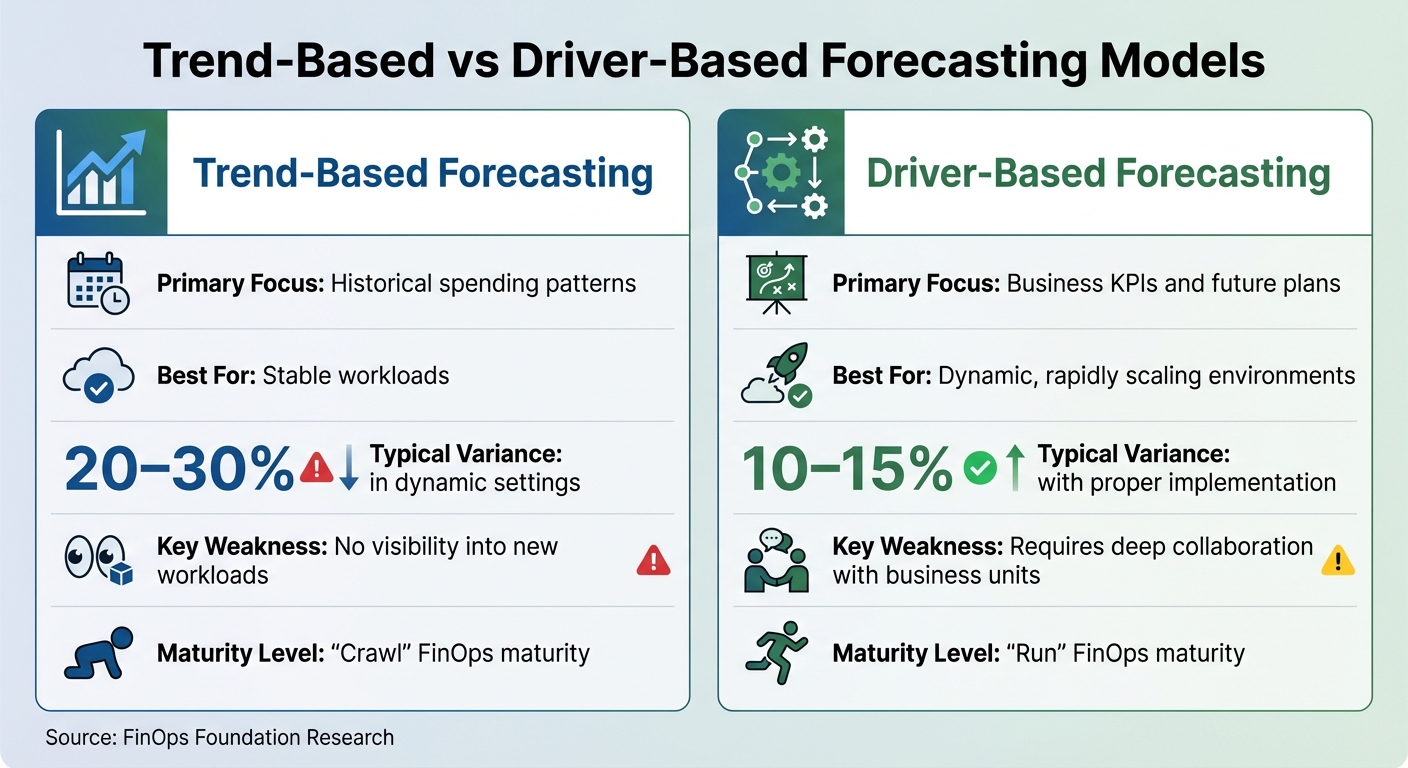 {Trend-Based vs Driver-Based Cloud Cost Forecasting Models Comparison}
:::
{Trend-Based vs Driver-Based Cloud Cost Forecasting Models Comparison}
:::
Trend-based forecasting offers a straightforward way to predict cloud costs. These univariate models use 12–18 months of historical billing data to identify spending patterns and project them into the future. By relying on consistent past growth, these models serve as an accessible entry point for organisations that are new to predictive analytics or operate with stable, predictable workloads.
How Trend-Based Models Work
To get started, historical billing data from cloud providers - like AWS Cost and Usage Reports, Azure Cost Management exports, or Google Cloud billing data - needs to be preprocessed. This involves filtering out anomalies, one-time purchases, and costs from deleted resources or expired subscriptions. Skipping this step can lead to skewed forecasts, as a single large purchase could distort the results. Techniques like exponential smoothing, ARIMA, or linear regression are then applied to generate cost predictions.
For example, AWS Cost Explorer uses an 80% prediction interval. If the historical data shows excessive volatility, the tool may not provide a forecast at all [6]. Reliable predictions typically require at least one complete billing cycle of data [6]. Additionally, adjustments for variations in month length are necessary to avoid artificial spikes in the data. When forecasting for a specific period, such as the next 12 months, it's important to align the historical look-back period to the same duration to capture seasonal trends [2]. This method establishes a foundation for understanding more advanced models designed for dynamic workloads.
Advantages and Limitations
While trend-based models are a useful tool for FinOps teams aiming to predict costs, they come with limitations, especially in fast-changing environments. These models work well in stable settings but struggle when workloads or market conditions shift unexpectedly. For example, in steady-state environments, the variance between predicted and actual spend might be around 20%. However, in dynamic scenarios, variances can climb as high as 70%. For FinOps teams at the Crawl
maturity level, a variance of roughly 20% is generally acceptable [7]. Traditional forecasting methods often fall within a 20–30% variance range [2].
A real-world example highlights these challenges: a video streaming company using trend-based forecasting reported cost variances ranging from 20% to 70%. The high variance occurred because the model couldn't account for net new
workloads absent from the historical data [2]. Since these models focus on past spending, they cannot anticipate sudden market changes, new product launches, or unexpected demand surges. When tools like AWS Cost Explorer display a wide prediction band, it's a sign of high historical volatility and reduced forecast reliability [6].
| Factor | Trend-Based Forecasting | Driver-Based Forecasting |
|---|---|---|
| Primary Focus | Historical spending patterns | Business KPIs and future plans |
| Best For | Stable workloads | Dynamic, rapidly scaling environments |
| Typical Variance | 20–30% in dynamic settings | 10–15% with proper implementation |
| Key Weakness | No visibility into new workloads [2] | Requires deep collaboration with business units [2] |
| Maturity Level |
CrawlFinOps maturity [7] |
RunFinOps maturity [7] |
Driver-Based Forecasting Models
Driver-based forecasting shifts the focus to future cost influences, emphasising business events and strategic decisions instead of relying solely on historical billing data. This method is particularly useful for organisations dealing with fluctuating workloads, frequent product launches, or unpredictable growth patterns.
Understanding Driver-Based Models
Driver-based models group cost influences into four key categories:
- Internal: Factors like product launches, feature rollouts, architectural changes, or Kubernetes configuration updates [10][11].
- External: Influences such as user growth, seasonal spikes, sales events, or market fluctuations [10][11].
- Strategic: Decisions involving regional expansions, mergers, or planned Savings Plans and Reserved Instances [10].
- Reverse: Elements like customer churn, optimisation efforts, or retired workloads [10][11].
A crucial aspect of these models is the use of unit economics to determine per-unit costs. For instance, a SaaS provider calculated that handling 1.5 million API calls per month cost £10,312.50, resulting in a unit cost of approximately £0.0068 per call. Using this metric, they forecasted that onboarding a new customer generating 2 million additional API calls would raise operating costs by about £13,650 [10].
This approach highlights the importance of structured collaboration and a thorough understanding of financial impacts when implementing driver-based forecasting.
Best Practices for Using Driver-Based Models
To make the most of driver-based forecasting, collaboration across teams is essential. Schedule quarterly meetings with Finance, Procurement, Product, and Sales teams to identify demand drivers, such as marketing campaigns or new growth initiatives [10][8]. Each driver should have:
- A quantified financial impact.
- A defined start date.
- A designated owner responsible for tracking and accountability [11].
For new deployments, tools like the AWS Pricing Calculator can help integrate cost estimates directly into your master forecast [10][8].
Start with a trend-based baseline to capture what's already in motion. Then layer in driver-based assumptions as they become known - ideally before they hit production.- Erik Peterson, AWS Optics Team Lead [11]
Hybrid Forecasting Strategies
Combining Trend and Driver-Based Models
When it comes to cloud cost forecasting, a hybrid strategy offers a well-rounded approach by blending trend-based and driver-based models. This method starts with trend-based predictions as the baseline and incorporates driver-based insights to account for events that historical data alone cannot predict. While trend models are effective for steady workloads, driver-based models focus on how specific business metrics - like active user accounts or units sold - impact cloud expenses, capturing outlier events such as product launches [7].
Organisations operating at the Run
maturity level can achieve a forecast variance of 12% or less by combining rolling, trend-based, and driver-based models [7]. The process begins with establishing a stable trend baseline, followed by driver-based adjustments for anticipated business events. Finally, pipeline forecasting is added to account for new workloads that lack historical data [2].
For workloads with no historical precedent, driver-based pipeline forecasting becomes essential to tighten variance control. Relying solely on trend-based models for new deployments often results in variances ranging from 20% to 70% [2]. To manage unexpected workload growth, organisations should include a management reserve in their annual forecasts [2]. This layered approach underscores the importance of precise metrics and routine reviews to maintain accuracy.
Key Metrics and Review Frequency for Hybrid Models
For hybrid forecasting to succeed, monitoring key metrics is crucial. Metrics such as Mean Absolute Percentage Error (MAPE) and Weighted Absolute Percentage Error (WAPE) are particularly useful for evaluating forecast accuracy [2][11]. WAPE is often favoured because it accounts for spend volume, ensuring that smaller accounts with high percentage variances do not disproportionately affect overall accuracy [11]. To avoid skewed variance reports, it’s critical to use amortised cost data, which factors in Reserved Instances and Savings Plans [11][3].
Variance thresholds vary by organisational maturity: Crawl
stage organisations aim for 20%, Walk
stage for 15%, and Run
stage for 12% [7][3]. Forecasts should be reviewed monthly or quarterly, with automated alerts set up to flag variances that exceed acceptable levels [3][8][11]. For services with high variability, such as AI workloads, weekly or even daily reviews are recommended to quickly address unexpected costs. In these cases, practitioners aim for a variance of no more than 5% from actual costs each month [4].
Tools and Benchmarks for Predictive Cloud Cost Forecasting
Comparing Predictive Analytics Tools
When it comes to managing cloud costs effectively, having the right tools and benchmarks is key. The choice of tool often depends on how advanced an organisation’s processes and technical capabilities are. For instance, AWS Cost Explorer is a great starting point for teams in the early stages of their cloud cost management journey. It’s free to use within the AWS Billing Console and can analyse up to 38 months of historical data while offering an 18-month forecast. This makes it ideal for spotting long-term trends and seasonal patterns. Plus, it provides AI-driven explanations in plain language, helping users understand cost trends better [13][6].
For organisations looking for more advanced features, Amazon QuickSight offers machine learning (ML)-powered forecasting. It includes options like customisable prediction intervals and what-if
scenario analysis. Pricing starts at £14 per month for an Enterprise Author licence, with Reader access costing £0.23 per session, capped at £3.90 monthly. This tool suits teams at the intermediate stage, often referred to as the Walk
level, and is particularly useful for creating forecasts across multiple business units or product lines [9].
At the high end of the spectrum, Amazon Forecast allows data analysts to train custom ML predictors using quantiles like P10, P50, and P90. Costs for training sessions range from £8 to £78 for enterprise customers [9]. Meanwhile, multi-cloud environments can benefit from tools like Cloudaware, which integrates Configuration Management Database (CMDB) data to deliver forecasts tailored to specific applications, teams, or environments [11]. Another strong contender is DoiT Cloud Analytics, which uses ML to handle seasonality and outliers across varying timeframes, from hourly to annual forecasts [12].
| Tool | Maturity Level | Primary KPI | Estimation Method |
|---|---|---|---|
| AWS Cost Explorer | Crawl | Total Spend / Service Spend | Historical Trend (80% Prediction Interval) |
| Amazon QuickSight | Walk | Custom KPIs (e.g., Unit Cost) | ML-based Time Series with What-IfAnalysis |
| Amazon Forecast | Run | Weighted Quantile Loss (wQL) | Custom ML Predictors (P10, P50, P90) |
| Cloudaware | Run | Variance by CMDB Scope | Driver-based + Trend-based Hybrid |
| DoiT | Walk/Run | Forecast per Grouping | ML with Seasonality & Outlier Handling |
These tools provide a strong foundation for evaluating forecast performance using standardised accuracy benchmarks.
Benchmarks for Forecast Accuracy
After selecting the right tool, it’s crucial to measure how accurate the forecasts are. Accuracy benchmarks typically evolve as an organisation's financial operations (FinOps) practices mature. For teams just starting out (Crawl
stage), a forecast variance of ±20–25% is a reasonable target. As processes become more refined (Walk
stage), this narrows to ±15%. Advanced teams in the Run
stage aim for a variance of ±10–12% [11].
Accuracy is usually measured using metrics like WAPE (Weighted Absolute Percentage Error) or MAPE (Mean Absolute Percentage Error). These metrics are especially helpful in identifying discrepancies before invoices arrive [11].
Forecast granularity also plays a pivotal role. Early-stage teams (Crawl
) often focus on forecasts at the cloud vendor or business unit level, with reviews conducted monthly. Intermediate teams (Walk
) refine their focus to individual business applications or products and review forecasts weekly. Advanced teams (Run
) achieve continuous, on-demand forecasting, breaking down costs at the account, project, or subscription level [2][11].
Research-Backed Best Practices and Business Outcomes
Empirical Outcomes from Predictive Analytics
Predictive analytics has proven to be a game-changer in cloud cost management, with research showing that advanced machine learning (ML) models outperform traditional methods by a significant margin. For instance, while manual approaches achieve only 58.2% accuracy, AI-driven systems deliver far superior results [5]. These advancements translate into tangible savings: organisations using AI-powered recommendation engines report an average 27% reduction in cloud costs within a year [5].
Real-world success stories highlight the impact of these technologies. Netflix, for example, implemented AI-based auto-scaling and predictive ML models to handle global streaming demand. This move cut resource waste by 50%, saving the company hundreds of millions annually [5]. Similarly, Arabesque AI used AI-powered analytics alongside Google Cloud's preemptible instances to dynamically scale their financial model training, slashing server costs by 75% [5]. Another standout, Airbnb, achieved a 27% reduction in cloud costs by employing predictive analytics to resize instances and balance workloads across AWS and Google Cloud during peak seasons [5]. These examples underscore the effectiveness of trend-based and driver-based models.
Beyond cost savings, predictive analytics boosts operational efficiency. AI-driven systems can cut cost analysis and remediation time by 68% and detect spending anomalies with 92.5% accuracy, compared to 63.7% for traditional methods [1]. Companies like Validity have leveraged these tools to reduce time spent on cloud cost administration by 90%, freeing up teams to focus on more strategic initiatives [5].
Additionally, mature organisations using predictive analytics achieve tighter forecast variances, as previously evidenced. These outcomes naturally lead to the importance of integrating forecasting with budgeting and real-time alerts for even greater efficiency.
Integrating Forecasting with Budgeting and Alerts
To maximise the benefits of predictive analytics, integrating forecasting with budgeting and real-time alerts is essential. Effective forecasting doesn't just predict costs - it actively informs spending controls. As the FinOps Foundation puts it, Good forecasts drive good business decisions
[2]. The best results occur when organisations establish a FinOps loop
, where Finance sets growth constraints, Engineering manages workload timing, and FinOps oversees a regular review process [11][2].
To monitor forecast accuracy, organisations should use metrics like WAPE (Weighted Absolute Percentage Error) or MAPE (Mean Absolute Percentage Error) to identify deviations early [11]. Real-time alerts should be set at multiple thresholds - typically 50%, 80%, and 100% of the budget - and should include forecasted-to-breach
signals sent via tools like Slack or Jira [11]. Erik Peterson, AWS Optics Team Lead, advises:
Run Budgets and Anomaly Detection together. One shows the trend. The other flags the surprise[11].
Including optimisation efforts in forecasts is equally critical for maintaining trust in the models. The FinOps Foundation highlights this point:
Optimization efforts must be included in forecasts to maintain trust in the model. Otherwise, variance will show up as unexplained[11].
This approach means treating activities such as rightsizing, reserved instance purchases, and savings plan commitments as dated deltas
in forecasts rather than unpredictable side effects. Skyscanner exemplifies this principle. By adopting AI-enhanced cost visibility, the company identified optimisation opportunities that generated enough savings in just two weeks to cover an entire year's platform licence [5]. Such integration solidifies predictive analytics as a cornerstone of strategic cloud cost management.
Conclusion and Next Steps
Key Takeaways
Predictive analytics has the power to turn cloud cost management into a proactive, data-driven process. Studies show that AI-driven forecasting models can achieve variances as low as 10–12% for organisations with a mature approach, compared to the much higher variances of 40–60% seen with traditional methods [11].
The best results come from using a hybrid approach that blends trend-based baselines with driver-based assumptions. This method captures both historical data and planned changes within the business. However, success isn't just about technology. It requires a coordinated effort involving Finance, Engineering, and FinOps teams, supported by regular variance reviews and automated alerts. Effective forecasts also need to account for optimisation efforts, like rightsizing, Reserved Instances, and Savings Plans, ensuring models remain accurate and trustworthy [11]. These principles lay the groundwork for a scalable and effective implementation strategy.
Implementing Predictive Analytics in Your Business
To put these insights into action, start by gathering 12–18 months of normalised billing data. This data will help establish a reliable trend-based baseline [11]. Segment forecasts by specific scopes, such as applications, teams, environments, or Kubernetes namespaces, to ensure clear ownership and accountability [11].
For businesses looking for expert guidance, Hokstad Consulting offers cloud cost engineering services. They can help you transition from manual forecasting to machine learning-driven systems that align with FinOps maturity standards. Their targets include ±20–25% variance at the Crawl level, ±15% at Walk, and ±10–12% at Run [11].
To scale these processes effectively, focus on creating repeatable workflows. Regularly review variance, categorise drivers into Internal, External, Strategic, and Reverse groups, and include management reserves in annual forecasts to handle the unpredictability of cloud scaling [11][2]. With a well-structured approach, predictive analytics can become a cornerstone of your cloud financial management strategy.
FAQs
How much data is needed to reliably forecast cloud costs?
Reliable cloud cost forecasting depends heavily on historical data that accurately represents workload patterns and usage trends. While the exact amount of data needed can differ, models operating in dynamic environments often show deviations of 40–60%. By blending long-term forecasts with real-time predictions, you can achieve much greater accuracy.
When should I use trend-based vs driver-based forecasting?
Trend-based forecasting relies on historical data to estimate future cloud costs. This approach works well for workloads that are steady and predictable or for long-term planning, such as setting annual budgets. However, it can falter when faced with unexpected changes or fluctuations.
Driver-based forecasting, on the other hand, focuses on specific business activities - like product launches or scaling operations. This makes it a better fit for dynamic and rapidly changing environments. By combining both methods, businesses can achieve a balance, maintaining stability while staying flexible enough to meet evolving demands.
How can I measure and improve forecast accuracy over time?
To get better at forecasting accuracy, focus on fine-tuning your data processing and modelling methods. Make good use of historical data and keep a close eye on variances and anomalies. Spotting these deviations allows you to tweak your models when necessary. Regular evaluations are key to keeping your forecasts precise and useful for decision-making.