
Managing Kubernetes costs can be tricky. Two tools - Horizontal Pod Autoscaler (HPA) and Cluster Autoscaler (CA) - help optimise resources, but they work at different levels. HPA scales pods based on demand, while CA adjusts the number of nodes in your cluster. Used together, they can significantly cut costs by ensuring resources match workload needs.
Here’s the key takeaway:
- HPA adjusts pod replicas based on metrics like CPU or custom demand indicators.
- CA adds or removes nodes when pods can’t be scheduled or nodes are underused.
- Together, they prevent wasted capacity while maintaining performance, potentially reducing costs by up to 70%.
If you’re running stateless apps or workloads with fluctuating traffic, combining these tools is your best bet for efficient scaling.
How HPA Reduces Costs
Scaling Based on Resource Metrics
Horizontal Pod Autoscaler (HPA) keeps an eye on resource usage in real time, ensuring that the number of pods matches the actual demand. Every 15 seconds, it checks metrics and compares the utilisation to pre-set targets [1]. If there's a mismatch, HPA calculates the required number of replicas using a simple formula:
desiredReplicas = ceil(currentReplicas * (currentMetricValue / desiredMetricValue)) [1][3].
This system avoids over-provisioning and under-utilisation by adjusting pod counts - scaling up during high demand and scaling down during quieter periods. To prevent unnecessary scaling actions, HPA includes a tolerance mechanism that ignores changes within a 10% margin [1].
Roman Arcea, GKE Product Manager, highlights that setting a CPU target at 50% can lead to increased costs [8]. Testing showed that raising the HPA CPU target from 50% to 70% reduced peak capacity needs from 22 CPUs to 12 CPUs - a 45% drop - while maintaining acceptable response times [8]. For web-facing applications, using metrics like requests per second or concurrency often results in better scaling than relying solely on CPU usage [3]. By focusing on precise metrics, HPA helps cut costs by minimising idle resources.
Cost Impact of Pod-Level Scaling
Efficient scaling ensures that only the required number of pods run at any given time. For instance, a food delivery app in June 2025 used queue length metrics to scale from 15 pods during peak hours to just 5 during off-peak periods (10 hours daily), saving £8 per day per cluster - adding up to £240 per month [10].
Saulius Mašnauskas from Cast AI emphasises the importance of fine-tuning scaling mechanisms:
The tighter your Kubernetes scaling mechanisms are configured, the lower the waste and costs of running your application[9].
Before enabling HPA, it's essential to profile pods using kubectl top. This step ensures that workloads are efficient because autoscalers can amplify inefficiencies. If pods are wasteful to begin with, scaling up only multiplies that waste [7]. By optimising individual pods first, HPA can deliver real savings rather than simply scaling inefficient workloads.
Need help optimizing your cloud costs?
Get expert advice on how to reduce your cloud expenses without sacrificing performance.
How Cluster Autoscaler Reduces Costs
Scaling Nodes to Match Pod Demand
Cluster Autoscaler keeps an eye out for pods stuck in a Pending
state due to insufficient resources. Every 10 seconds, it scans for unschedulable pods [12]. When it spots them, it prompts the cloud provider to add more nodes, ensuring you don't waste money on idle, unused standby instances.
This process isn't one-way. Cluster Autoscaler also identifies underutilised nodes - those where the total pod resource requests fall below a set threshold, typically 50% by default [13]. It then shifts pods to other nodes and shuts down the underused ones. As Kubecost puts it:
Cluster Autoscaler plays a vital role in a Kubernetes cluster by ensuring adequate computing resources are available by adding nodes to a cluster and keeping infrastructure costs down by removing nodes[12].
A node is considered unneeded
if it stays underutilised for 10 minutes [13]. By consolidating resources, Cluster Autoscaler ensures you're only paying for active infrastructure. Unlike the Horizontal Pod Autoscaler (HPA), which reacts to real-time CPU and RAM usage, Cluster Autoscaler bases its decisions on pod requests - the reserved capacity each pod claims it needs.
Cost Savings Through Node-Level Optimisation
The node adjustment process is key to cutting unnecessary expenses. Moving from static overprovisioning to dynamic scaling can lead to 40–70% savings on infrastructure costs [2]. Cluster Autoscaler enables a pay-as-you-go approach, scaling down resources during low-demand periods.
Bin packing plays a crucial role here. Working with the Kubernetes scheduler, it ensures pods are packed onto the fewest nodes necessary, increasing resource density. This reduces the total number of nodes, allowing the autoscaler to quickly identify and terminate nodes that are empty or nearly empty. The least-waste expander further optimises this by selecting node groups that minimise unused CPU and memory [14].
For even more savings, alternative pricing models like Spot instances can be leveraged. Managed through Cluster Autoscaler, Spot instances can cut costs by up to 90% compared to On-Demand pricing [6][14]. By configuring node groups to use Spot instances for workloads that can tolerate interruptions and reserving On-Demand instances for critical services, you can strike a balance between reliability and cost efficiency. As noted in Kubernetes documentation:
The overall Node utilisation in a cluster can be used as a proxy for how cost-effective the cluster is[11].
While HPA focuses on optimising costs at the pod level, Cluster Autoscaler takes it a step further by improving efficiency at the infrastructure level. Together, they form a key part of a broader cost optimisation strategy.
Kubernetes Scaling Guide (2025): HPA, Cluster Autoscaler & More
HPA vs. Cluster Autoscaler: Direct Comparison
::: @figure 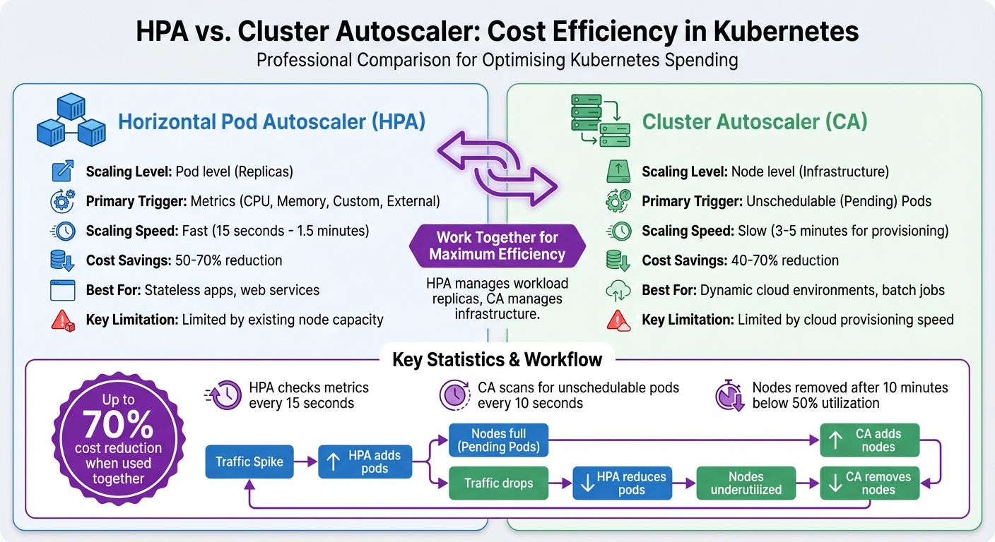 {HPA vs Cluster Autoscaler: Key Differences and Cost Savings Comparison}
:::
{HPA vs Cluster Autoscaler: Key Differences and Cost Savings Comparison}
:::
The Horizontal Pod Autoscaler (HPA) and Cluster Autoscaler tackle scaling from different angles. HPA adjusts the number of pod replicas based on resource metrics like CPU, memory, or even custom indicators such as request rates or queue lengths, focusing on the application level. On the other hand, the Cluster Autoscaler operates at the infrastructure level, modifying node counts when pods are stuck in a Pending
state due to insufficient resources. As Daniele Polencic from Learnk8s puts it:
The Cluster Autoscaler doesn't look at memory or CPU available when it triggers the autoscaling. Instead, \[it\] reacts to events and checks for any unschedulable Pods.[4]
One major distinction is scaling speed. HPA has a quick response time, with a 15-second control loop that enables it to handle sudden traffic spikes efficiently. Cluster Autoscaler, however, is slower, often taking 3–5 minutes to provision new virtual machines. This delay can lead to initial provisioning gaps if not carefully accounted for [4].
When it comes to cost management, the two offer different benefits. HPA provides granular savings by reducing pod replicas during low activity periods, while Cluster Autoscaler achieves broader savings by decommissioning entire underutilised nodes. Essentially, HPA optimises what’s running, whereas Cluster Autoscaler ensures the infrastructure is right-sized. These approaches complement each other: HPA minimises over-provisioning with faster scaling, while Cluster Autoscaler eliminates idle node costs.
Comparison Table: Cost Optimisation Features
| Feature | Horizontal Pod Autoscaler (HPA) | Cluster Autoscaler (CA) |
|---|---|---|
| Scaling Granularity | Pod level (Replicas) | Node level (Infrastructure) |
| Primary Trigger | Metrics (CPU, Memory, Custom, External) | Unschedulable (Pending) Pods |
| Resource Utilisation | Optimises pod-level allocation | Optimises cluster-wide node density |
| Prerequisites | Metrics Server, Resource Requests defined | Cloud provider integration, Node groups |
| Scaling Speed | Fast (seconds to ~1.5 minutes) | Slow (3–5 minutes for node provisioning) |
| Cost-Saving Potential | 50–70% reduction [2] | 40–70% reduction [2] |
| Primary Limitation | Limited by existing node capacity | Limited by cloud provisioning speed |
| Best Use Case | Stateless apps, web services | Dynamic cloud environments, batch jobs |
The interplay between HPA and Cluster Autoscaler is crucial. HPA depends on the Cluster Autoscaler to ensure there’s enough physical capacity to handle increased traffic, while the Cluster Autoscaler relies on HPA (or similar tools) to generate the demand required to justify scaling nodes up or down. Without this synergy, you risk stranded pods waiting for resources or idle nodes draining your budget. Understanding these roles helps determine how to best use each autoscaler in different scenarios.
When to Use HPA or Cluster Autoscaler
Choose HPA when your cluster already has spare capacity, and opt for Cluster Autoscaler when scaling physical nodes is necessary to meet demand. Here's a closer look at when each autoscaler works best for managing costs effectively.
When to Use HPA
HPA works best when your cluster has unused capacity. In these cases, HPA can quickly add pods to existing nodes without triggering the expense of scaling up nodes themselves [3][4]. This method maximises the utilisation of your current infrastructure.
Applications that are stateless and can scale horizontally - like web servers, REST APIs, or microservices - are ideal for HPA [3][5]. These workloads benefit from HPA’s ability to adapt to changing traffic patterns within seconds. Using custom metrics, such as request rate or queue depth, allows for precise scaling decisions, avoiding delays caused by pods being marked as 'Pending' [3][10][4]. However, relying solely on memory usage as a scaling metric is less effective. Memory pressure tends to linger, making scale-down events slower and less impactful for cost savings [3].
If your pods outgrow the cluster’s current capacity, that’s where Cluster Autoscaler comes into play.
When to Use Cluster Autoscaler
While HPA focuses on scaling pods, Cluster Autoscaler manages node-level adjustments to reduce idle infrastructure costs. If nodes operate below 50% utilisation for over 10 minutes, CA can remove them, ensuring you only pay for active resources [2][15]. This feature is particularly beneficial in cloud environments with pay-as-you-go models, such as AWS, GCP, or Azure [2].
Cluster Autoscaler is an excellent fit for batch jobs and workloads with unpredictable spikes [2]. If HPA tries to add pods but there aren’t enough physical resources to accommodate them, CA steps in to provision extra nodes [3][16]. Without CA, HPA alone could result in pending pods and service disruptions.
For instance, a fashion e-commerce business successfully combined latency-based HPA with Cluster Autoscaler, using spot and Arm64 instances. This approach reduced their compute costs by 42%, scaling their cluster from 40 nodes during sales events down to just 8 nodes in quieter periods [5].
Using HPA and Cluster Autoscaler Together
Combining Horizontal Pod Autoscaler (HPA) and Cluster Autoscaler (CA) creates a dynamic, efficient scaling system that adapts to workload demands. Here's how it works: when application load increases, HPA adds more pods. If existing nodes can't handle these new pods, CA steps in to provision additional nodes. Conversely, as demand decreases, HPA reduces the number of pods, leaving nodes underutilised. CA then removes these idle nodes, cutting unnecessary costs [2][19].
This division of tasks - short-term pod scaling by HPA and node-level capacity management by CA - ensures smooth operations. HPA reacts quickly to demand spikes, often within 15 seconds, while CA adjusts the infrastructure within a few minutes to maintain the right capacity [17]. Without this coordination, the system risks inefficiencies: HPA alone could leave pods pending if nodes are full, while CA alone might result in static pod counts that waste resources during quieter times [2][16]. By working together, these tools optimise both cost and resource use, regardless of fluctuating demand.
The financial benefits are clear. When configured correctly, this synergy can significantly reduce costs. For example, CA can leverage Spot instances - cheaper, short-term nodes - to support HPA's scaled workloads, offering savings of up to 90% on compute costs [2][18]. However, proper setup is crucial. Use Pod Disruption Budgets to prevent simultaneous node removals that could disrupt services [2][6]. Also, avoid using HPA and Vertical Pod Autoscaler (VPA) on the same metric, as this can cause conflicts, with HPA adding pods while VPA increases pod size, leading to instability [2][17].
Valdas Rakutis from Cast AI emphasises this coordinated approach:
To achieve cost savings for workloads that experience regular changes in demand, use HPA in combination with cluster autoscaling. This will help you reduce the number of active nodes when the number of pods decreases.[16]
This combination is especially effective for stateless applications with variable traffic, such as microservices, web APIs, and event-driven backends [2][19]. Considering that only 13% of requested CPU in Kubernetes clusters is typically utilised, and just 20% to 45% of requested resources power actual workloads, this dual-layer strategy directly tackles resource over-provisioning [18].
Best Practices for Cost-Efficient Configuration
Setting Resource Requests and Limits
Getting resource requests and limits right is key to efficient autoscaling. Set requests too high, and you'll waste capacity. Set them too low, and you risk performance issues or scheduling failures. A smart way to strike the balance is the 90th percentile rule: analyse resource usage over two weeks and set requests at the 90th percentile[5]. This method ensures your pods have enough room for regular operations without over-provisioning.
Tuning resource settings can lead to noticeable savings. For instance, increasing an HPA CPU target from 50% to 70% reduced provisioned resources by 84% while handling the same workload[8]. For memory, aim for 75–80% utilisation to leave enough headroom and avoid out-of-memory errors[5]. Similarly, setting CPU targets in the 60–70% range provides room for sudden spikes without unnecessary scaling[5].
Other key settings include configuring minReplicas to maintain a baseline and maxReplicas to cap costs[2]. For the Cluster Autoscaler, adjusting the scale-down-utilisation-threshold - typically set at 50% - can help improve node density[2]. Using the least-waste expander can further refine how nodes are selected for scaling[6][2].
Once you've set these configurations, keep an eye on them. Workloads evolve, and continuous monitoring is essential to maintain efficiency.
Monitoring and Adjusting Configurations
Even with well-planned configurations, regular monitoring is crucial to sustaining cost-efficiency. Autoscaling delays - from HPA adjustments to cloud provider provisioning - can take 6.5 to 7 minutes[4]. To counter this lag, you can use low-priority pause
pods (PriorityClass -1) as placeholders. These pods can be preempted by real workloads, allowing immediate scaling while the Cluster Autoscaler provisions new nodes[4][3].
Scaling should also reflect metrics tied to actual user demand. For web services, metrics like requests per second (RPS) or queue length often align more closely with load than CPU usage alone[3][2]. For example, a fashion e-commerce company cut its monthly compute costs by 42% by using latency-based HPA targets, Cluster Autoscaler with spot instances, and rightsizing memory requests[5]. Additionally, consolidating node groups into fewer, larger pools can improve efficiency by reducing idle resources and ensuring nodes run closer to full capacity[6].
When combined, these practices enhance both HPA and Cluster Autoscaler performance, forming a solid foundation for cost-effective scaling.
Conclusion
Optimising both the application and infrastructure layers using the Horizontal Pod Autoscaler (HPA) and Cluster Autoscaler (CA) is a smart way to cut Kubernetes costs. HPA dynamically adjusts pod replicas based on real-time demand, while CA scales nodes up or down to match capacity needs. Together, they turn static setups into a flexible, pay-as-you-go system, potentially reducing cluster costs by 25–40% during the initial rollout[5].
Understanding your workload patterns is crucial. Begin by profiling your applications over a two-week period to fine-tune resource requests and limits. Stateless web services and APIs typically benefit most from HPA, while CA ensures nodes expand or shrink appropriately, avoiding both resource bottlenecks and unused capacity. For UK businesses, where energy costs and currency fluctuations can hit hard, precise autoscaling configurations are vital to keep infrastructure costs strictly tied to actual usage.
FAQs
What metrics should I use for HPA besides CPU?
When evaluating performance, don't just focus on CPU usage. Metrics like memory usage, the ratio of resource requests to actual usage, and network egress are equally important. These insights can help fine-tune resource allocation and keep costs under control.
Why are my pods Pending even with HPA enabled?
Pods can end up in a Pending state when using Horizontal Pod Autoscaler (HPA) if the cluster lacks enough resources, like CPU or memory. Another common culprit is improperly set resource requests and limits, which can block scheduling altogether. While HPA dynamically adjusts the number of pod replicas based on metrics, it doesn’t handle adding new nodes to the cluster.
If the Cluster Autoscaler isn’t set up correctly or is restricted by factors like node limits, pods won’t get scheduled and will remain Pending. To address this, keep a close eye on resource availability and ensure the autoscaler is properly configured.
How do I tune requests and limits for cheaper autoscaling?
To manage autoscaling costs effectively in Kubernetes, it's crucial to set precise resource requests and limits for your pods. This ensures the Horizontal Pod Autoscaler (HPA) can make smarter scaling decisions, avoiding unnecessary over-provisioning or performance bottlenecks. Regularly monitor CPU and memory usage to align resource requests with typical workload patterns. Additionally, incorporating multiple metrics and stabilisation windows can help avoid unpredictable scaling behaviours, leading to better resource efficiency and cost savings.