If I want tighter cloud forecasts, I track four KPIs first: forecast accuracy, MAPE, forecast bias, and budget variance. Then I check the inputs behind them: allocation coverage, commitment use, waste, anomaly response, forecast ownership, update speed, and engineering follow-through.
In plain terms, the article says this: a forecast is only as good as the billing data, cost allocation, and review process behind it. It also makes a clear split between budget, rolling forecast, and actual spend, and it recommends measuring on net amortised spend in £. For most teams, the target is to keep monthly forecast error around ±5–10% for stable production work, while more volatile workloads may sit closer to ±15–20%.
Here’s the short version of what matters:
- Start with clean data from AWS, Azure, and GCP in one view
- Measure forecast accuracy directly with:
- Forecast Accuracy %
- MAPE
- Forecast Bias (MPE)
- Budget Variance %
- Check forecast quality drivers, including:
- Cost allocation coverage
- Unit economics
- Commitment coverage and utilisation
- Cloud waste %
- Anomaly detection speed
- Track process discipline with:
- Forecast coverage by team or service
- Time to update after change
- Engineering participation
- Time to remediation
- Use one dashboard to compare forecast, budget, and actuals by team, service, and environment
- Review on a set cadence: daily for anomalies, weekly for drift, monthly for finance checks, and quarterly for commitment planning
A few figures stand out. The piece flags unallocated spend above 5% as a problem, suggests anomaly detection inside 24 hours with fixes inside 72 hours, and notes that shutdown schedules for non-essential environments can cut those costs by 40–65%. It also says firms with a structured forecasting process can bring budget variance down from 25–40% to under 10%.
::: @figure 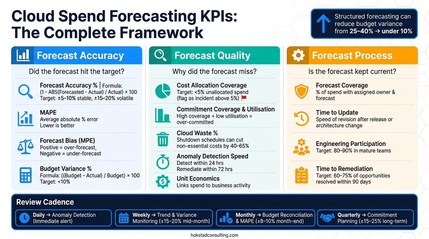 {Cloud Spend Forecasting KPIs: Accuracy, Quality & Process at a Glance}
:::
{Cloud Spend Forecasting KPIs: Accuracy, Quality & Process at a Glance}
:::
Forecasting Cloud Costs FinOps FOCUS and Power BI
Need help optimizing your cloud costs?
Get expert advice on how to reduce your cloud expenses without sacrificing performance.
Quick comparison
| KPI group | What I use it for | Main signals |
|---|---|---|
| Accuracy KPIs | Check if the forecast was right | Forecast Accuracy %, MAPE, MPE, Budget Variance |
| Quality KPIs | Find why the forecast missed | Allocation coverage, unit economics, commitments, waste, anomalies |
| Process KPIs | Keep the forecast current | Ownership, update time, engineering input, remediation time |
If I had to sum the article up in one line, it would be this: good cloud forecasting is part maths, part clean data, and part team discipline.
KPIs that directly measure forecast accuracy
These KPIs work best when you calculate them on net amortised spend, split between production and non-production. That split matters more than it might seem at first glance. Non-production spend often jumps around due to shutdown schedules, so mixing it with production can mask problems in your production forecast [1].
Forecast accuracy rate and error bands
Forecast accuracy rate shows how close your predicted spend was to actual spend:
Forecast Accuracy % = (1 - ABS(Forecasted Spend - Actual Spend) / Actual Spend) * 100
For stable production setups, a monthly forecast error of ±5–10% is a sensible target. More volatile workloads, such as AI model training or setups tied to fast product launches, may need wider bands of ±15–20% [3].
Run these KPI calculations on net amortised spend.
MAPE and forecast bias
MAPE (Mean Absolute Percentage Error) shows the average absolute forecast error as a percentage of actual spend. In plain terms, it tells you how far off your forecast was on average, without caring whether you were too high or too low [3].
Forecast bias, measured as Mean Percentage Error (MPE), shows whether your forecasts tend to lean in one direction. A positive MPE means you are over-forecasting. A negative MPE means you are under-forecasting. Looking at MAPE and MPE together helps you see both the size of the miss and the pattern behind it [3].
Budget variance and forecast volatility
Once you know the forecast error, the next step is to see whether it is causing budget drift or unstable projections.
Budget variance compares actual spend with the fixed financial plan, not the rolling forecast:
Budget Variance % = ((Budget - Actual) / Budget) * 100
This is mainly a finance control metric. It tells you whether spend stayed inside the agreed plan, rather than whether the forecast itself was right [2][4].
Forecast volatility shows how much your forward forecast shifts between planning cycles. Big week-to-week changes often point to uncertain inputs or changing demand [2]. A weekly review of actuals against the rolling forecast can help you spot drift early [3].
| Metric | Formula | Primary Use |
|---|---|---|
| Forecast Accuracy % | (1 - ABS(Forecasted - Actual) / Actual) * 100 |
Measuring prediction reliability [4] |
| Budget Variance % | ((Budget - Actual) / Budget) * 100 |
Financial accountability and compliance [4] |
| Burn Rate | Actual Spend / Time Period |
Tracking how quickly budget is being consumed [4] |
KPIs that improve forecast quality
These KPIs show why a forecast missed and what to fix next. They answer three plain questions: is the data complete, are discounts and waste under control, and are spikes spotted fast? That’s what makes forecast accuracy easier to explain.
Cost allocation coverage and unit economics
Cost allocation coverage measures the share of total spend assigned to a cost centre, product, team or environment. If spend sits unallocated, the baseline for every forecast gets weaker. Treat unallocated spend above 5% as an incident.
Once allocation is in good shape, unit economics link cloud spend to business activity. That makes it easier to break forecasts down with more precision by product, environment, team or customer.
When spend is allocated cleanly, the next check is simple: are committed capacity and waste under control?
Commitment utilisation and cloud waste percentage
Two KPIs matter here, and they work best when read together:
- Commitment coverage - the share of eligible usage covered by commitments
- Commitment utilisation - the share of committed capacity actually used
Coverage shows how much usage gets a discount. Utilisation shows how much of the committed capacity is being used. If coverage is high but utilisation is low, you’ve over-committed and are paying for capacity that sits unused [5]. Commitment gaps and waste can warp the cost base your model is trying to predict.
Cloud waste percentage measures avoidable idle or underused spend. Automated shutdown schedules for non-essential environments can cut the cloud costs tied to them by 40–65% [1].
Cost anomaly detection accuracy
Anomaly detection helps protect forecast quality over time. If anomalies slip through, they skew the history your next forecast will lean on.
Run Budgets and Anomaly Detection together. One shows the trend. The other flags the surprise.- Erik Peterson, AWS Optics Team Lead [2]
Aim to detect issues within 24 hours and remediate them within 72 hours. Set alerts at 50%, 80% and 100% of forecasted spend.
The next section shifts from model quality to process discipline across teams and services.
Process KPIs that keep forecasts current
After you measure forecast accuracy, the next step is to track the process KPIs that keep those forecasts up to date. Accuracy doesn't come from maths alone. It also depends on how the work is run day to day. If ownership is fuzzy, updates slip, or engineering teams aren't involved, the forecast starts to drift.
Forecasting coverage across teams and services
Forecasting coverage measures the share of cloud spend with an assigned owner and forecast at application, team or namespace level, so alerts have a clear owner [2].
Time to update forecasts after a change
Ownership matters. But speed matters too. A forecast that isn't revised after a release, architecture change, or pricing change can become misleading fast. Time-to-update tracks how quickly the forecast is revised once a major change goes live.
A simple way to keep this moving is to combine a 30-minute weekly variance check with monthly forecast refreshes involving finance, engineering and FinOps [2][3].
Engineering engagement and time to remediation
The last process check is simple: do teams act on what the forecast is showing? Track the share of engineering teams that take part in cost reviews and optimisation work - aim for 80–90% participation in mature teams [6] - alongside time to remediation, which measures the gap between identifying an opportunity and putting the fix in place.
You should also aim to deliver 60–75% of identified opportunities within 90 days [6].
Using KPI dashboards to make better FinOps decisions
How to combine KPIs into one reporting view
To make these KPIs useful day to day, bring them into a single dashboard. Group the metrics into accuracy, quality and process layers. That way, the main signals sit in one view, and it becomes much easier to compare forecast, budget and actual spend side by side.
Show forecast, budget and actual in £ by team, service and environment, and use DD/MM/YYYY throughout. It also helps to set clear variance flags: ±15–20% in the middle of the month, then ±8–10% by month-end [7].
| Review Level | Frequency | Primary Focus | Acceptable Variance |
|---|---|---|---|
| Operational | Daily | Anomaly detection & usage spikes | Immediate alert |
| Tactical | Weekly | Trend analysis & variance monitoring | ±15–20% (Mid-month) |
| Financial | Monthly | Budget reconciliation and MAPE | ±8–10% (Month-end) |
| Strategic | Quarterly | Commitment planning & long-term roadmap | ±15–25% (Long-term) |
Then add known business events on top. Campaigns and migrations should be logged as manual inputs, not treated as model noise. That simple step can cut avoidable forecast swings, which often feed bias and volatility [7].
Where expert cloud cost engineering can help
Hokstad Consulting can help build dashboards, automate reporting and tighten allocation data.
Conclusion: the KPIs that matter most
Once the dashboard is live, start with forecast accuracy rate, MAPE, forecast bias and budget variance. Those are the core measures. From there, improve forecast quality by tracking cost allocation coverage, unit economics, commitment utilisation and cloud waste percentage.
To keep forecasts current, monitor coverage, update speed, engineering engagement and remediation time as well. Organisations that put a structured forecasting approach in place can cut budget variance from 25–40% to under 10% [7].
FAQs
Which KPI should I prioritise first?
Prioritise tagging-related KPIs first. Tagging sits at the heart of cloud cost management. Without it, resources slip out of sight, and forecasts, chargebacks, and budget reports start to drift off course.
Start with Percentage of Tagging Policy Compliance and Percentage of Untagged Cloud Resources. Once you’ve got that visibility in place, move on to metrics like Budget Variance and Forecast Accuracy.
Why use net amortised spend for forecasting?
Using net amortised spend gives you a steadier, more accurate view of actual cloud consumption. It blends raw usage costs with the amortisation of long-term commitments, such as Reserved Instances and Savings Plans, while leaving out taxes and refunds.
That matters because it strips out the spikes caused by upfront payments. As a result, it’s easier to line up cloud spend with finance-approved budgets and build forecasts around the value of resources used over time.
How often should cloud forecasts be reviewed?
Cloud forecasts need regular reviews if you want them to stay accurate as business conditions shift.
In practice, run weekly variance reviews to compare spend with budget. Then add formal monthly and quarterly assessments on top. This gives you a steady rhythm to test assumptions, update models with the latest usage data, and factor in issues like currency fluctuations.