
Forecasting cloud spend is key to better budgeting and resource planning. Rising costs make accurate predictions essential for UK businesses to avoid overspending and ensure efficient use of resources. Time series models, such as ARIMA, SARIMA, and Prophet, analyse past data to predict future trends, helping finance and engineering teams make informed decisions.
Key Takeaways:
- Why Forecast? Predicting cloud spend can improve savings plan effectiveness by 15–25% and help maintain budget accuracy within ±10–12%.
- Models to Know:
- ARIMA: Best for non-seasonal, stable trends. Requires stationary data and manual tuning.
- SARIMA: Adds seasonal capabilities, ideal for predictable cycles like monthly or quarterly patterns.
- Prophet: Handles complex, calendar-driven data with minimal preprocessing, perfect for irregular spikes or events.
- Accuracy Goals: Achieve a MAPE below 15% for reliable forecasts.
- Steps to Start:
Quick Comparison:
| Model | Best For | Seasonality Handling | Ease of Use | Accuracy (MAPE) |
|---|---|---|---|---|
| ARIMA | Stable, non-seasonal trends | None | Moderate (manual) | 8–15% |
| SARIMA | Predictable seasonal cycles | Strong (single cycle) | Moderate (complex) | 10–18% |
| Prophet | Irregular spikes, calendar events | Strong (multi-cycle) | High (automated) | 6–12% |
Use these models to forecast cloud costs effectively, reduce budget variances, and optimise savings plans.
::: @figure 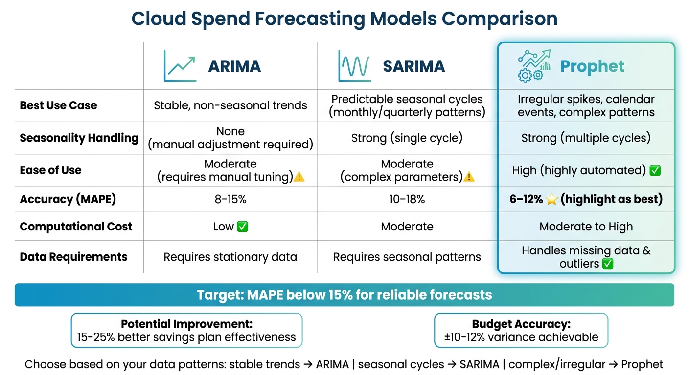 {ARIMA vs SARIMA vs Prophet: Cloud Spend Forecasting Models Comparison}
:::
{ARIMA vs SARIMA vs Prophet: Cloud Spend Forecasting Models Comparison}
:::
No-Code Time Series Forecasting (Multivariate AutoML on GCP)
Need help optimizing your cloud costs?
Get expert advice on how to reduce your cloud expenses without sacrificing performance.
ARIMA Models for Cloud Spend Forecasting
ARIMA, or AutoRegressive Integrated Moving Average, is a widely used time-series forecasting model, particularly effective for predicting non-seasonal cloud spending patterns. By identifying and capturing the relationships within your data, ARIMA can help forecast future expenses when seasonal fluctuations aren't a significant factor [4]. The model works by converting non-stationary data into a stationary series using a differencing technique, enabling more accurate predictions.
This approach is ideal for trends like steady growth in infrastructure costs or gradual savings from optimisation efforts. However, if your cloud expenditure follows clear cycles (e.g., weekly or monthly), a seasonal model like SARIMA might be a better fit.
ARIMA Parameters Explained
ARIMA models are governed by three key parameters: p, d, and q. Here's how each contributes to forecasting cloud spend:
| Parameter | Component | Role in Cloud Spend Forecasting |
|---|---|---|
| p | Autoregressive (AR) | Uses previous cloud spend values to predict future costs |
| d | Integrated (I) | Specifies how many differencing steps are needed to stabilise trends |
| q | Moving Average (MA) | Adjusts predictions by considering past forecasting errors |
For instance, if p = 2, the model uses the last two months' cloud spending to predict the next month. A d = 1 setting means the data is differenced once to make it stationary, while q refines the forecast by integrating past errors. Tools like AutoARIMA or Google Cloud's ARIMA_PLUS can automate parameter selection, often choosing configurations based on the Akaike Information Criterion (AIC) [5].
Once the parameters are set, you can apply ARIMA to your cloud spend data for actionable insights.
Using ARIMA with Cloud Spend Data
To start, gather detailed billing data from platforms like AWS, Azure, or GCP. Aggregate this data to a consistent frequency (daily or monthly) that matches your forecasting needs [1][2].
Before applying ARIMA, clean and prepare your data:
- Exclude anomalies: Remove one-off charges like migration fees or upfront Reserved Instance payments to avoid skewing trends.
- Handle missing data: Use interpolation to fill gaps.
- Address variance: Apply transformations such as logarithmic or Box-Cox if variance is high.
- Check stationarity: Use the KPSS test to confirm if the data is stationary. If not, apply first-order differencing (d = 1) [7].
Once the data is ready, fit the ARIMA model using either manually chosen parameters or automated tools [5][6]. After fitting, validate the model by analysing its residuals - if they resemble white noise (random, uncorrelated fluctuations), the model is effectively capturing patterns. For medium-term forecasts, aim for a Mean Absolute Percentage Error (MAPE) below 15% [2].
Hokstad Consulting applies these techniques to help UK businesses forecast cloud spending with precision, enabling better cost control and infrastructure planning.
SARIMA Models for Seasonal Cloud Spend
While ARIMA is great for identifying trends and short-term patterns, it often struggles when cloud spending exhibits regular seasonal cycles. That's where SARIMA (Seasonal AutoRegressive Integrated Moving Average) comes in. SARIMA builds on ARIMA by adding a seasonal component, making it ideal for handling both gradual trends and predictable fluctuations - like December's retail boom or the provisioning spikes that often occur at the end of a quarter [8].
The main advantage of SARIMA lies in its ability to capture recurring seasonal patterns. Unlike ARIMA, which primarily compares one month to the previous, SARIMA also looks at corresponding periods from earlier cycles. This makes it better equipped to handle long-term, repeating trends and provides a more accurate forecast for cloud spend [8].
Understanding Seasonality in Cloud Spend
Seasonality in cloud spending refers to patterns that occur at consistent intervals. These might include:
- Monthly billing cycles, where costs peak on renewal dates.
- Quarterly increases tied to business reporting periods.
- Weekly usage spikes driven by customer activity.
If these cycles aren't accounted for, forecasts might miss key peaks or misinterpret seasonal dips as random fluctuations [10]. SARIMA tackles this issue using seasonal differencing (D), which removes seasonal effects by comparing values from one complete cycle apart - like this month's spend compared to the same month last year [8]. This approach helps isolate and model the recurring patterns.
SARIMA Parameters Explained
SARIMA models are expressed as SARIMA(p, d, q)×(P, D, Q)s. The lowercase parameters represent the non-seasonal ARIMA component, while the uppercase parameters handle seasonal patterns [10]. The s parameter specifies the length of the seasonal cycle. For example:
- Use s = 12 for monthly billing cycles.
- Use s = 7 for daily data with weekly patterns.
- Use s = 52 for weekly data reflecting annual cycles [9].
| Parameter | Component | Role in Cloud Spend Forecasting |
|---|---|---|
| P | Seasonal AR | Links current spend to the same period in previous cycles (e.g., last December). |
| D | Seasonal Differencing | Removes seasonal effects by comparing data from one full cycle ago. |
| Q | Seasonal MA | Adjusts for recurring forecast errors at the seasonal lag. |
| s | Seasonal Period | Defines the cycle length (e.g., 12 for monthly, 7 for weekly, or 52 for annual weekly patterns). |
Once a SARIMA model is fitted, it’s important to check the autocorrelation function (ACF) of the residuals. If significant lags remain at multiples of the seasonal period (like 12 or 24 for monthly data), it means the model hasn’t fully captured the seasonal signal. Start with minimal differencing - both non-seasonal (d = 0 or 1) and seasonal (D = 0 or 1) - to avoid over-differencing, which can erase useful patterns and increase forecast variance [10].
Prophet for Flexible Cloud Spend Forecasting
Prophet offers a practical approach to forecasting cloud spending, especially when compared to ARIMA or SARIMA. Unlike these models, Prophet doesn’t require intensive parameter tuning or strict adherence to stationarity. Developed by Meta, it’s specifically designed to handle business data with strong calendar patterns - just like cloud spend metrics. Prophet’s additive model breaks down data into four key components: trend, seasonality (using Fourier series to account for daily, weekly, and yearly cycles), holidays, and noise. One standout feature is its ability to automatically detect changepoints, which helps identify sudden shifts in spending caused by events like product launches or pricing adjustments. It’s also resilient to missing data and outliers, making it well-suited for handling the unpredictable nature of cloud billing. Prophet accommodates both linear and logistic trends; if you choose logistic, you can set a cap to ensure forecasts stay within budget limits or infrastructure constraints. Additionally, you can encode known events, such as Black Friday, as holidays to capture multi-day spending surges [11].
Prophet Model Features
Prophet’s real advantage lies in its ability to break down cloud spending into understandable parts. Here’s how it works:
- Trend (g(t)): Tracks long-term changes, whether it’s steady growth due to increased cloud adoption or a decline following cost-optimisation efforts.
- Seasonality (s(t)): Captures recurring patterns, such as lower activity on weekends or higher usage at the end of a financial quarter.
- Holidays (h(t)): Accounts for anticipated disruptions, like Black Friday traffic spikes or planned system migrations.
- Error (e(t)): Represents unpredictable factors, such as unplanned outages or untracked
shadow IT
usage.
This decomposition makes Prophet particularly effective when cloud spending is highly variable or influenced by specific calendar events [11].
When to Use Prophet for Cloud Spend
Prophet shines in scenarios where cloud spending data is shaped by complex calendar-driven changes or sudden structural shifts. It’s ideal for situations involving significant usage spikes tied to specific dates, such as promotional campaigns, seasonal traffic increases, or scheduled migrations. On the other hand, if your cloud spending follows a stable, straightforward pattern with clear autocorrelation and minimal seasonal complexity, models like ARIMA or SARIMA might provide more accurate results. Ultimately, selecting the right model depends on the specific characteristics of your data [11].
Comparing ARIMA, SARIMA, and Prophet
This section pits ARIMA, SARIMA, and Prophet against each other to help you decide which forecasting model suits your cloud spend patterns and available expertise. Each model has its strengths and limitations, so understanding these can guide your choice.
ARIMA is a solid choice for simple, non-seasonal datasets. However, it requires manual tuning and works best with stationary data. SARIMA builds on ARIMA by incorporating the ability to handle seasonal patterns, like monthly billing cycles, but comes with a steeper learning curve due to its complexity. On the other hand, Prophet is designed to simplify forecasting. It can handle intricate business trends, holidays, and even missing data, making it particularly appealing for teams without deep statistical knowledge.
Accuracy Comparison
Accuracy is a key factor when choosing a model. Here's how the three models compare based on performance metrics:
- Prophet leads the pack with a Mean Absolute Error (MAE) of 0.74, far outclassing SARIMA (2.18) and ARIMA (3.02) [16].
- For seasonal data, Prophet's Root Mean Square Error (RMSE) stands at 52.02 [14], and its Mean Absolute Percentage Error (MAPE) ranges between 6–12% [2]. In comparison, SARIMA's RMSE hits 77.20, and ARIMA's MAPE falls between 8–15%.
Practical Considerations
When it comes to computational cost and usability, the models vary:
- ARIMA runs efficiently with minimal resources but demands expert tuning to achieve accurate results.
- SARIMA is more resource-intensive and requires a deeper understanding of statistical modelling due to its parameter complexity.
- Prophet, while needing relatively more processing power, automates much of the forecasting process. Tools like Ray can significantly speed up Prophet’s computations, achieving up to a 300% improvement on standard hardware [15]. For teams with limited data science expertise, Prophet's automation is a major advantage.
As data science writer Kishan A puts it:
Prophet simplifies forecasting by automating many steps... making it a go-to option for non-experts[13].
Choosing the Right Model
The best approach is to start simple and scale up as your data needs grow. For stable and predictable workloads, begin with basic techniques like moving averages before exploring ARIMA or Prophet [2]. If your cloud spend fluctuates due to irregular events - like seasonal traffic spikes, promotional campaigns, or planned migrations - Prophet is better equipped to handle these complexities. Regardless of the model, aim for a MAPE below 15% to ensure reliable medium-term cloud budgeting [2].
Model Performance Comparison
| Model | Accuracy (MAPE) | Seasonality Handling | Computational Cost | Ease of Use |
|---|---|---|---|---|
| ARIMA | Moderate (8–15% MAPE) | None (manual adjustment) | Low | Moderate (requires tuning) |
| SARIMA | High (10–18% MAPE) | Strong (single cycle) | Moderate | Moderate (parameter complexity) |
| Prophet | High (6–12% MAPE) | Strong (multiple cycles) | Moderate to High | High (highly automated) |
Evaluating and Deploying Forecast Models
Model Validation and Diagnostics
Before rolling out any forecast model, it's essential to confirm its performance. Start with residual analysis to examine the errors left after fitting the model. If you notice patterns in these residuals, it suggests the model hasn't fully captured the underlying signals in the data [17].
To ensure the errors are random (or white noise
), pair residual analysis with the Ljung-Box test [17][20]. For an added layer of confidence, use backtesting: train the model on historical data, then test it on a reserved dataset. This approach helps gauge how well the model performs on unseen data, minimising risks before committing actual budgets [17].
Accuracy metrics like MAPE (Mean Absolute Percentage Error), RMSE (Root Mean Square Error), and Bias are critical for evaluating forecast reliability [2]. For context, advanced FinOps teams usually aim to keep forecast variances within ±10–12% [3]. However, remember that data quality plays a massive role - around 62% of forecasting errors are linked to poor input data. Ensuring clean, high-quality data is non-negotiable [17].
Deployment Best Practices
Once forecasts are validated, focus on a smooth deployment process. Automate the deployment pipeline with integrated monitoring tools (such as Slack or Jira) to flag deviations greater than 15% in real-time [2][19]. This proactive monitoring allows teams to address issues before month-end invoices arrive. Additionally, instead of forecasting a single overall figure, break down models by specific cost drivers - like EC2 families, Kubernetes nodes, or product teams - for more granular insights [19].
Maintaining data quality doesn't stop at the preparation phase. During deployment, continue monitoring inputs and update your strategies to reflect new patterns. Regularly retrain models - monthly or quarterly - to account for changes in system architecture. Be cautious with validation methods: sequential validation is essential for time series data to prevent data leakage, as methods like k-fold cross-validation are unsuitable here [2][18]. To avoid misinterpreting known events (like Black Friday sales or planned migrations) as anomalies, maintain a business event calendar [2].
For cloud commitments, use the lower bound of the 95% confidence interval to avoid overcommitting resources [2]. Instead of relying on a single figure, create multiple scenarios - pessimistic, baseline, and optimistic - to prepare for business fluctuations [2][12]. This structured approach can reduce budget variances from 25–40% to under 10% while boosting commitment utilisation by 15–25% [2].
Conclusion
Forecasting cloud expenses effectively means selecting a model that aligns with your data and business needs. ARIMA works well for stable, short-term predictions but depends on data stationarity and fine-tuning. SARIMA builds on this by incorporating seasonal trends, making it ideal for businesses with predictable monthly or quarterly cycles. Meanwhile, Prophet, developed by Meta, is designed to handle missing data, outliers, holiday effects, and intricate seasonal patterns with minimal preprocessing [21][22].
- ARIMA: Best for steady, consistent usage [2].
- SARIMA: Suited for clear seasonal cycles [21].
- Prophet: Ideal for volatile, migration-heavy, or long-term forecasts [22].
Matching your chosen model to your specific cloud usage patterns is crucial for accurate results.
Key Takeaways
To refine your forecasting process, think of it as climbing a model ladder.
Start with simpler techniques like moving averages, move on to ARIMA for stable workloads, and finally, consider Prophet or machine learning for more complex scenarios [2]. This step-by-step approach avoids unnecessary complexity while enhancing your forecasting capabilities.
Here are a few practical tips:
- Data Quality Matters: Achieve 85–95% tagging coverage before diving into detailed forecasting. This alone can boost accuracy by 20–30% [2].
- Keep a Business Event Calendar: Mark key events like product launches or migrations to ensure they aren’t misinterpreted as anomalies [2].
- Savings Plans and Reserved Instances: Commit to 90% of the lower bound of your forecast to strike a balance between securing discounts and avoiding overcommitment [2].
Structured forecasting can significantly improve financial outcomes. Organisations adopting these models often reduce budget variance from 25–40% to under 10% [2]. Whether managing a £500,000 annual cloud budget or scaling into the millions, the right forecasting approach transforms cloud spending from a challenge into a well-optimised investment aligned with your business goals.
For expert advice on tailoring your cloud spend forecasting strategy, visit Hokstad Consulting at https://hokstadconsulting.com.
FAQs
How much historical billing data is needed for a reliable cloud spend forecast?
To build a dependable cloud spend forecast, you should review at least 12 months of past billing data. This helps you spot important trends and seasonal fluctuations, leading to more precise predictions.
How do I include savings plans, reserved instances, and one-off charges in the model?
To ensure your cloud spend forecasting is accurate, it's important to account for savings plans, reserved instances, and one-off charges as separate cost elements.
- Reserved instances and savings plans: These are relatively predictable and can be treated as fixed or semi-fixed costs in your forecasts.
- One-off charges: Expenses like migrations or upgrades are less predictable and should be categorised as anomalies or occasional spikes.
By segmenting costs into these categories and applying tailored forecasting models, you can achieve better precision and maintain greater control over your budget.
What should I do when a forecast suddenly becomes inaccurate after a migration or pricing change?
When a forecast goes off track following a migration or pricing adjustment, it's crucial to revise your forecasting models to align with the updated circumstances. Incorporate scenario planning to anticipate potential outcomes, closely track actual costs against your forecasts, and double-check the reliability of your data sources.
Leverage AI-driven tools, such as What-If models, to dynamically simulate the effects of these changes. Consistent reviews, setting up alerts, and fostering collaboration across teams can help fine-tune assumptions and ensure your forecasts stay accurate, even in the face of shifting conditions.